Analyzing discharge at Kings Creek

Introduction

This vignette demonstrates several preMetabolizer utilities for working with daily streamflow records. We use kings_discharge, a built-in dataset that contains daily USGS discharge and water temperature for Kings Creek (monitoring location USGS-06879650) at the Konza Prairie Biological Station in northeastern Kansas during water year 2025 (2024-10-01 through 2025-09-30).

Kings Creek is a well-studied tallgrass prairie stream with a highly episodic flow regime: many days record zero discharge, with brief but intense pulses following rainfall events.

library(preMetabolizer)
library(dplyr)
#> 
#> Attaching package: 'dplyr'
#> The following objects are masked from 'package:stats':
#> 
#>     filter, lag
#> The following objects are masked from 'package:base':
#> 
#>     intersect, setdiff, setequal, union
library(ggplot2)

Load and reshape the data

data(kings_discharge)
glimpse(kings_discharge)
#> Rows: 716
#> Columns: 5
#> $ monitoring_location_id <chr> "USGS-06879650", "USGS-06879650", "USGS-0687965…
#> $ time                   <date> 2024-10-01, 2024-10-01, 2024-10-02, 2024-10-02…
#> $ value                  <dbl> 0.0, 19.5, 0.0, 18.2, 0.0, 22.0, 0.0, 21.7, 0.0…
#> $ parameter_code         <chr> "00060", "00010", "00060", "00010", "00060", "0…
#> $ qualifier              <chr> "", "", "", "", "", "", "", "", "", "", "", "",…

The data are in long format with one row per date × parameter combination. We pivot to wide format so each row represents a single day with discharge (00060, cfs) and water temperature (00010, °C) as separate columns.

kings <- kings_discharge |>
  tidyr::pivot_wider(
    id_cols = time,
    names_from = parameter_code,
    values_from = value
  ) |>
  rename(discharge_cfs = `00060`, temp_C = `00010`)

glimpse(kings)
#> Rows: 365
#> Columns: 3
#> $ time          <date> 2024-10-01, 2024-10-02, 2024-10-03, 2024-10-04, 2024-10…
#> $ discharge_cfs <dbl> 0, 0, 0, 0, 0, 0, 0, 0, 0, 0, 0, 0, 0, 0, 0, 0, 0, 0, 0,…
#> $ temp_C        <dbl> 19.5, 18.2, 22.0, 21.7, 22.7, 21.1, 18.1, 18.9, 19.4, 19…

Convert units

USGS reports discharge in cubic feet per second (cfs). convert_flow() converts between cfs, cubic meters per second (cms), and liters per second (lps). For comparison with international literature we add a cms column.

kings <- kings |>
  mutate(discharge_cms = convert_flow(discharge_cfs, from = "cfs", to = "cms"))

summary(kings[, c("discharge_cfs", "discharge_cms")])
#>  discharge_cfs      discharge_cms    
#>  Min.   : 0.00000   Min.   :0.00000  
#>  1st Qu.: 0.00000   1st Qu.:0.00000  
#>  Median : 0.00000   Median :0.00000  
#>  Mean   : 0.08759   Mean   :0.00248  
#>  3rd Qu.: 0.00000   3rd Qu.:0.00000  
#>  Max.   :25.10000   Max.   :0.71075

Add season

get_season() assigns a meteorological season (Winter, Spring, Summer, Fall) to each date, which is useful for stratified summaries and plots.

kings <- kings |>
  mutate(season = factor(
    get_season(time),
    levels = c("Winter", "Spring", "Summer", "Fall")
  ))

count(kings, season)
#> # A tibble: 4 × 2
#>   season     n
#>   <fct>  <int>
#> 1 Winter    89
#> 2 Spring    93
#> 3 Summer    94
#> 4 Fall      89

Time series overview

kings |>
  tidyr::pivot_longer(
    c(discharge_cms, temp_C),
    names_to = "variable",
    values_to = "value"
  ) |>
  mutate(variable = recode(
    variable,
    discharge_cms = "Discharge (m³/s)",
    temp_C = "Temperature (°C)"
  )) |>
  ggplot(aes(time, value)) +
  geom_line(linewidth = 0.4) +
  facet_wrap(~variable, ncol = 1, scales = "free_y") +
  labs(x = NULL, y = NULL) +
  theme_bw()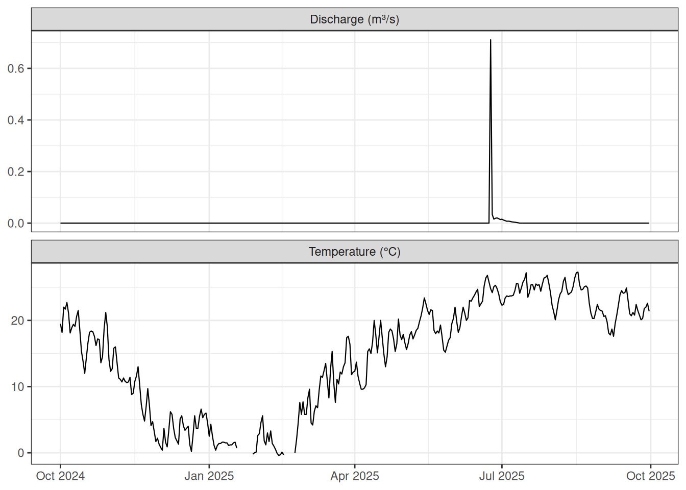

Flag anomalous values

flag_z() uses a moving-window robust Z-score to identify values that deviate unusually from their local neighborhood. Here we apply it to water temperature to check for sensor spikes or data-entry errors.

z_result <- flag_z(kings$temp_C, width = 7, threshold = 3, return_z = TRUE)

kings <- kings |>
  mutate(
    temp_z = z_result$z,
    temp_flag = z_result$flag
  )

cat(
  "Flagged temperature values:",
  sum(!is.na(kings$temp_flag)),
  "\n"
)
#> Flagged temperature values: 9

Flow duration curve

A flow duration curve (FDC) shows what fraction of time discharge equals or exceeds a given value. calc_exceedance_prob() implements the Weibull plotting-position formula. Setting rm.zero = TRUE excludes days with zero discharge from the ranking, so the curve reflects the non-zero portion of the flow regime.

kings <- kings |>
  mutate(exceed_prob = calc_exceedance_prob(discharge_cms, rm.zero = TRUE))

zero_pct <- mean(kings$discharge_cms == 0, na.rm = TRUE) * 100
cat(sprintf("Days with zero discharge: %.1f%%\n", zero_pct))
#> Days with zero discharge: 95.1%

kings |>
  filter(!is.na(exceed_prob)) |>
  ggplot(aes(exceed_prob, discharge_cms, color = season)) +
  geom_point(size = 1.5, alpha = 0.8) +
  scale_x_continuous(
    labels = \(x) paste0(round(x * 100), "%"),
    limits = c(0, 1)
  ) +
  scale_y_log10() +
  scale_color_manual(values = c(
    Winter = "#4575b4",
    Spring = "#74add1",
    Summer = "#fdae61",
    Fall   = "#d73027"
  )) +
  labs(
    x     = "Exceedance probability",
    y     = "Discharge (m³/s)",
    color = "Season"
  ) +
  theme_bw()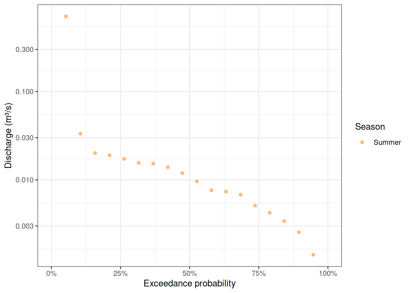

Discharge variability by season

calc_cv() computes the coefficient of variation (CV), a normalized measure of variability. A high CV indicates a flashy, episodic regime; a low CV indicates more stable baseflow conditions.

kings |>
  filter(discharge_cms > 0) |>
  group_by(season) |>
  summarise(
    n_days   = n(),
    mean_cms = mean(discharge_cms, na.rm = TRUE),
    cv_pct   = calc_cv(discharge_cms, na.rm = TRUE, as_percent = TRUE),
    .groups  = "drop"
  )
#> # A tibble: 1 × 4
#>   season n_days mean_cms cv_pct
#>   <fct>   <int>    <dbl>  <dbl>
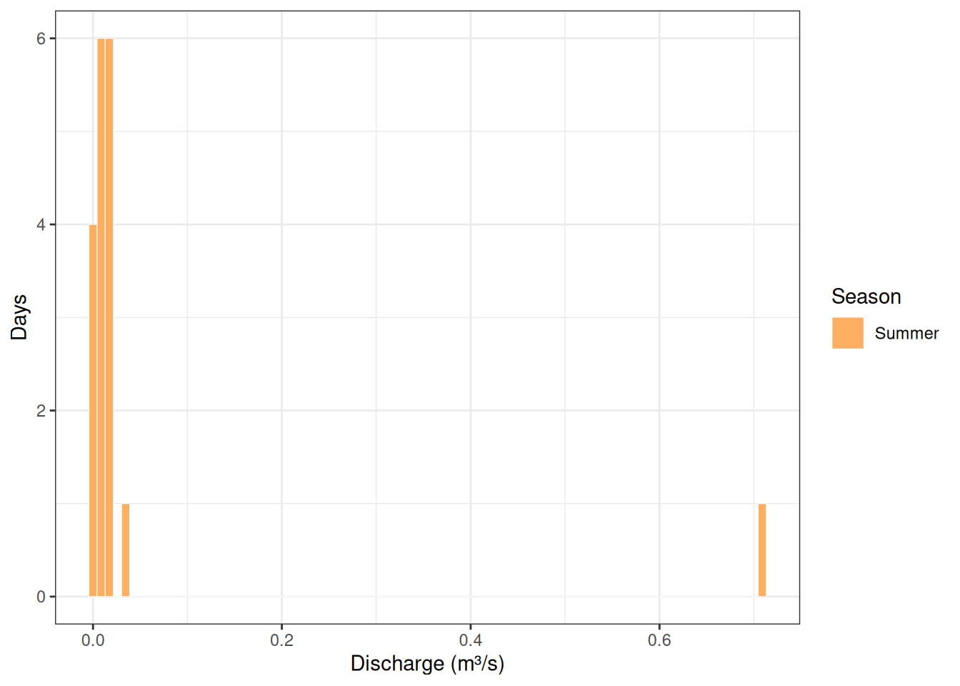
#> 1 Summer     18   0.0503   328.

Discharge histogram

calc_bin_width() suggests a histogram bin width using classical rules. The "fd" (Freedman-Diaconis) method is robust to outliers and works well for right-skewed flow data.

non_zero_q <- kings |> filter(discharge_cms > 0)

bw <- calc_bin_width(non_zero_q$discharge_cms, method = "fd")

ggplot(non_zero_q, aes(discharge_cms, fill = season)) +
  geom_histogram(binwidth = bw, color = "white", linewidth = 0.2) +
  scale_fill_manual(values = c(
    Winter = "#4575b4",
    Spring = "#74add1",
    Summer = "#fdae61",
    Fall   = "#d73027"
  )) +
  labs(
    x    = "Discharge (m³/s)",
    y    = "Days",
    fill = "Season"
  ) +
  theme_bw()