Introduction
preMetabolizer includes small physical-property and unit-conversion helpers for common hydrology and atmospheric science tasks. These functions return plain numeric vectors, making them easy to use in base R, dplyr pipelines, and model input tables.
Flow conversions
convert_flow() converts discharge between cubic feet per second ("cfs"), cubic meters per second ("cms"), and liters per second ("lps").
flow <- tibble::tibble(discharge_cfs = c(1, 5, 25, 100)) |>
  mutate(
    discharge_cms = convert_flow(discharge_cfs, from = "cfs", to = "cms"),
    discharge_lps = convert_flow(discharge_cfs, from = "cfs", to = "lps")
  )

flow
#> # A tibble: 4 × 3
#>   discharge_cfs discharge_cms discharge_lps
#>           <dbl>         <dbl>         <dbl>
#> 1             1        0.0283          28.3
#> 2             5        0.142          142.
#> 3            25        0.708          708.
#> 4           100        2.83          2832.
Pressure conversions and elevation correction
convert_pressure() converts barometric pressure between common units. correct_bp() adjusts pressure from a weather station elevation to a site elevation.
convert_pressure(101.325, from = "kPa", to = "atm")
#> [1] 1
convert_pressure(1013.25, from = "hPa", to = "Pa")
#> [1] 101325

correct_bp(
  station_bp = 101.3,
  air_temp = 15,
  station_elev = 300,
  site_elev = 500,
  from_units = "kPa",
  to_units = "kPa"
)
#> [1] 98.92626
Elevation correction is useful when a nearby weather station is not at the same elevation as a stream site.
site_pressure <- tibble::tibble(
  station_bp_kPa = c(101.3, 100.9, 100.5),
  air_temp_C = c(15, 17, 18),
  station_elev_m = 300,
  site_elev_m = 500
) |>
  mutate(
    site_bp_kPa = correct_bp(
      station_bp = station_bp_kPa,
      air_temp = air_temp_C,
      station_elev = station_elev_m,
      site_elev = site_elev_m
    )
  )

site_pressure
#> # A tibble: 3 × 5
#>   station_bp_kPa air_temp_C station_elev_m site_elev_m site_bp_kPa
#>            <dbl>      <dbl>          <dbl>       <dbl>       <dbl>
#> 1           101.         15            300         500        98.9
#> 2           101.         17            300         500        98.6
#> 3           100.         18            300         500        98.2
Water density and water height
calc_water_density() calculates pure-water density from temperature. calc_water_height() converts pressure-sensor readings into water height.
temps <- tibble::tibble(water_temp = seq(0, 30, by = 5)) |>
  mutate(density_kg_m3 = calc_water_density(water_temp))

temps
#> # A tibble: 7 × 2
#>   water_temp density_kg_m3
#>        <dbl>         <dbl>
#> 1          0         1000.
#> 2          5         1000.
#> 3         10         1000.
#> 4         15          999.
#> 5         20          998.
#> 6         25          997.
#> 7         30          996.
For vented sensors, sensor_kPa is already the pressure from the water column. For unvented sensors, provide atmospheric pressure so it can be subtracted from the absolute sensor pressure.
water_level <- tibble::tibble(
  sensor_kPa = c(18.9, 19.2, 19.5),
  atmo_kPa = c(101.1, 101.0, 100.9),
  water_temp = c(14.8, 15.0, 15.2)
) |>
  mutate(
    vented_height_m = calc_water_height(
      sensor_kPa = sensor_kPa,
      water_temp = water_temp,
      type = "vented"
    ),
    unvented_height_m = calc_water_height(
      sensor_kPa = sensor_kPa + atmo_kPa,
      atmo_kPa = atmo_kPa,
      water_temp = water_temp,
      type = "unvented"
    )
  )

water_level
#> # A tibble: 3 × 5
#>   sensor_kPa atmo_kPa water_temp vented_height_m unvented_height_m
#>        <dbl>    <dbl>      <dbl>           <dbl>             <dbl>
#> 1       18.9     101.       14.8            1.93              1.93
#> 2       19.2     101        15              1.96              1.96
#> 3       19.5     101.       15.2            1.99              1.99
Modeled light
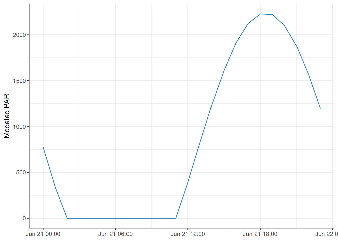
calc_par() estimates photosynthetically active radiation (PAR) from solar time and site coordinates. Input times should be mean solar time.
utc <- seq(
  as.POSIXct("2024-06-21 00:00:00", tz = "UTC"),
  as.POSIXct("2024-06-21 23:00:00", tz = "UTC"),
  by = "hour"
)

light <- tibble::tibble(
  dateTime_UTC = utc,
  solar_time = convert_to_solar_time(utc, longitude = -96.6)
) |>
  mutate(
    light_PAR = calc_par(
      solar_time = solar_time,
      latitude = 39.1,
      longitude = -96.6
    )
  )

head(light)
#> # A tibble: 6 × 3
#>   dateTime_UTC        solar_time          light_PAR
#>   <dttm>              <solar_dt>              <dbl>
#> 1 2024-06-21 00:00:00 2024-06-20 17:33:36      787.
#> 2 2024-06-21 01:00:00 2024-06-20 18:33:36      355.
#> 3 2024-06-21 02:00:00 2024-06-20 19:33:36        0
#> 4 2024-06-21 03:00:00 2024-06-20 20:33:36        0
#> 5 2024-06-21 04:00:00 2024-06-20 21:33:36        0
#> 6 2024-06-21 05:00:00 2024-06-20 22:33:36        0